ALLPCB


Overview
I reviewed medical image data loading and preprocessing methods recently and summarized them here. For applying deep learning to medical image analysis, such as lesion detection, tumor or organ segmentation, the first step is to understand the data. For medical image segmentation—for example abdominal organ segmentation or liver tumor segmentation—two main knowledge areas are needed: (1) medical image preprocessing methods, and (2) deep learning. The first area is necessary for the second because you need to know what kind of data is fed into the network.
This article describes common medical image loading methods and preprocessing techniques.
1. Medical Image Data Loading
1.1 ITK-SNAP
ITK-SNAP is a visualization tool for intuitively inspecting 3D medical image structures and can also be used for segmentation and bounding-box annotation. It is free and widely used. The ITK-SNAP official download page is available. Mango is another lightweight visualization tool that can be tried. I generally use ITK-SNAP.
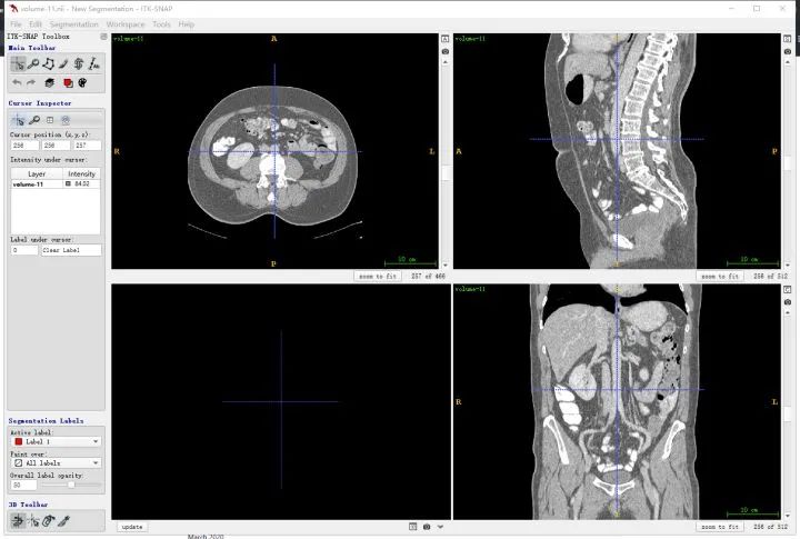
It is important to clarify anatomical directions. The three viewer panes correspond to three orthogonal planes, indexed as shown below. For example, the upper-left pane corresponds to the R-A-L-P orientation, which is the plane viewed from feet to head (the z direction).

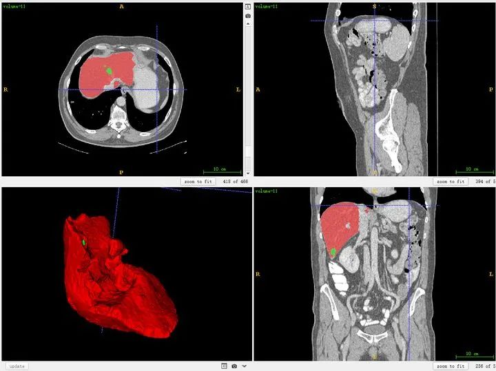
You can also load segmentation results to compare against images.
Public datasets are generally well annotated. Manual annotation follows a similar workflow. If the display is unclear or contrast is low, adjust window width and window level in the software.
1.2 SimpleITK
The most common medical images are CT and MRI, which are 3D and more complex than 2D images. Saved data can have many formats, for example .dcm, .nii(.gz), .mha, .mhd(+raw). These formats can be processed with Python's SimpleITK; pydicom can be used to read and modify .dcm files.
The goal of loading is to extract tensor data from each patient. Using SimpleITK to read .nii data as an example:
import numpy as np
import os
import glob
import SimpleITK as sitk
from scipy import ndimage
import matplotlib.pyplot as plt # import required libraries
# specify the data root path; the data directory contains volumes and the label directory contains segmentations, both in .nii format
data_path = r'F:LiTS_datasetdata'
label_path = r'F:LiTS_datasetlabel'
dataname_list = os.listdir(data_path)
dataname_list.sort()
ori_data = sitk.ReadImage(os.path.join(data_path,dataname_list[3])) # read one volume data
data1 = sitk.GetArrayFromImage(ori_data) # extract the array from the image
print(dataname_list[3],data1.shape,data1[100,255,255]) # print data name, shape and a specific element value
plt.imshow(data1[100,:,:]) # visualize the 100th slice
plt.show()
['volume-0.nii', 'volume-1.nii', 'volume-10.nii', 'volume-11.nii',...
volume-11.nii (466, 512, 512) 232.0
This indicates the data shape is (466,512,512).
Note the order is z,x,y. z is the slice index. x and y are the width and height of a slice. Plot result for z index 100: 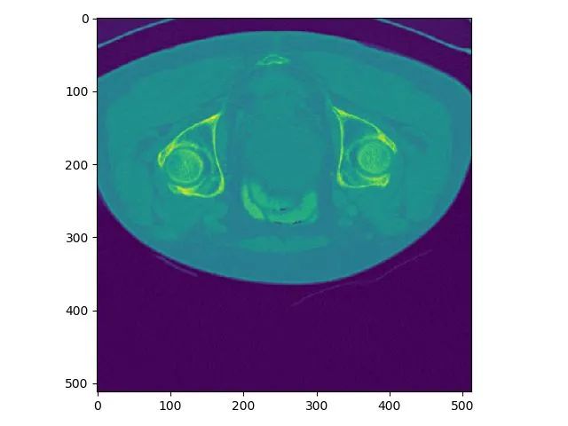
In ITK-SNAP the same slice is shown at coordinates (x,y,z) = (256,256,101) because ITK-SNAP uses 1-based indexing by default.
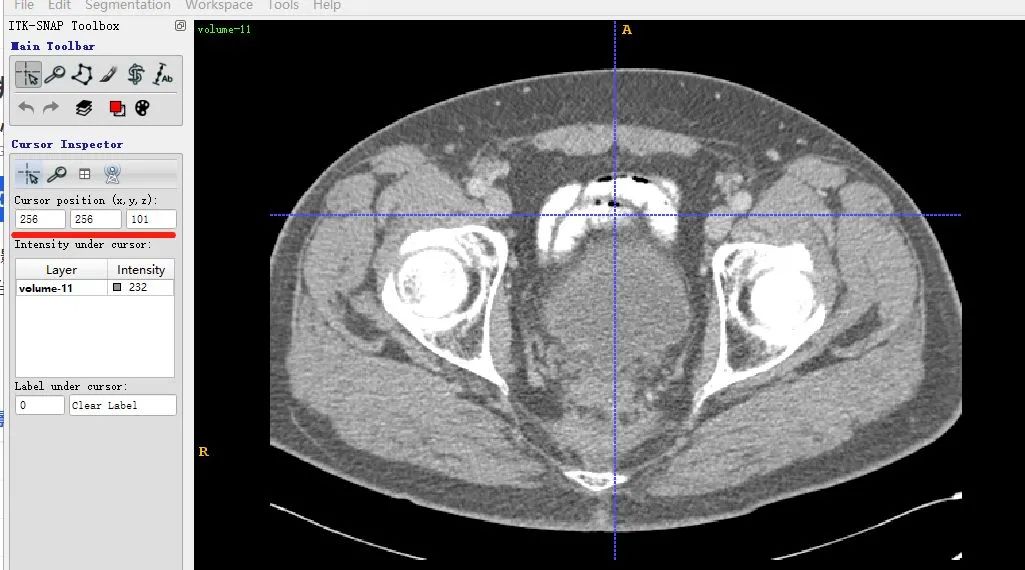
The X axes match between the two displays, but the Y axis is flipped due to differences in matplotlib display conventions. This does not indicate a mismatch in the loaded data.
2. Medical Image Preprocessing
Preprocessing methods vary by task and dataset, but the basic idea is to make the processed data more suitable for network training. Many 2D image preprocessing techniques can be adapted, such as contrast enhancement, denoising, and cropping. In addition, specific priors for medical images can be used, for example different Hounsfield unit ranges in CT correspond to different tissues and organs.
Based on the table above, raw data can be normalized:
MIN_BOUND = -1000.0
MAX_BOUND = 400.0
def norm_img(image): # normalize pixel values to (0,1) and clip out-of-range values to the boundaries
    image = (image - MIN_BOUND) / (MAX_BOUND - MIN_BOUND)
    image[image > 1] = 1.
    image[image < 0] = 0.
    return image
Data can also be standardized / zero-centered to shift the data mean to the origin:
image = image-meam
The normalization above applies to most datasets. Other preprocessing choices, such as the MIN_BOUND and MAX_BOUND values, are often dataset-dependent and it is useful to consult the preprocessing used in influential open-source implementations.
Save preprocessed datasets locally to reduce resource usage during training. Data augmentations like random cropping and affine transforms are typically applied during training.